Some months ago I attended a presentation where one of my colleagues, Panos, showed how he used Python to process data in a meaningful way. In particular, he showed how he extracted some interesting findings from a .csv file coming from the Boston Mayor’s 24 Hour Constituent Service web site. Such findings involved incidents that were still open by then, how many incidents were closed in a justifiable amount of time and others.

Since I am a little bit obsessed with computer security, I immediately started thinking of how I could do something similar in my field. So I wrote some scripts to query the “Web Hacking Incident Database”, which is a project dedicated to maintaining a list of web applications related to security incidents. Therefore, the aim of this post is twofold: a) you will see how you can process data in an elegant way and b) some findings on the hacking incidents of the past years.

The “Web-Hacking-Incident-Database” project, provides a .csv file containing major attack incidents for the past ten years. For every incident, there is also some valuable accompanying information that includes the date it took place, the attack method that it was used, the software error that possibly led to the attack, the country of the attacked entity and others.

There are numerous Python libraries that can be used to easily analyze data. In this experiment I used pandas, an open source, BSD-licensed library. A simple script that counts how many incident were mass attacks (typically targetting more than one entities) is the following:

import pandas

all_items = pandas.read_csv('test.csv')

mass = all_items[all_items['Mass Attack'] == 'Yes']

print len(mass)


The result was 62 out of 1365 records. Truth to be told, I had to handle the .csv file before feeding it as an argument to the read_csv method. This is because there were some inexplicable blank lines within some records. With a little help from my friend Vassilios, I wrote a script that removed such lines, thus making the file suitable.

To find the top five attack methods the following code fragment can be used:

print all_items['Attack Method'].value_counts()[:5]


This returns the following methods: Unknown (222), Denial of Service (DoS) (116), SQL Injection (115), Cross-Site Scripting (XSS) (40), Stolen Credentials (19). Interestingly, for a large number of incidents we do not know the attack method. The other methods is reasonable to appear on the top five since they have been topping the vulnerability lists of numerous bulletin providers for several years (OWASP Top Ten, CWE Top 25). In a similar manner, we can see that the top attacked entities are associated with governments (137), finance (64), retail (58), media (46) and entertainment (44).

You can also combine more than one condition with the “&” operator. For instance, to print the number of incidents that targeted U.S. government entities (15) you need to write something like the following:

in_goverments = all_items['Attacked Entity Field'] == 'Government'

in_usa = all_items['Attacked Entity Geography'] == 'USA'

print len(all_items[in_goverments & in_usa])


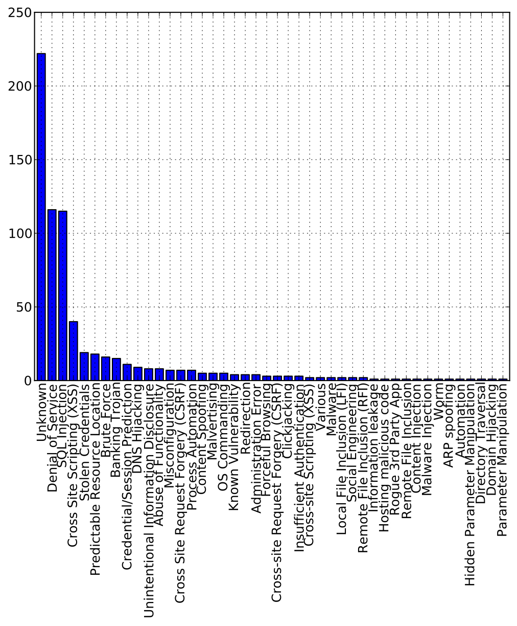
The number of the attack methods used.

Finally, it is easy to create plots like the one that can be seen above, which shows the corresponding number for all attack methods:

toa = all_items['Attack Method'].value_counts().plot(kind = 'bar')

fig = toa.get_figure()

fig.savefig('figure.pdf', bbox_inches='tight')


For more information on how you can use pandas you can refer to this link. There is also this interesting book that emphasizes how you can use Python to solve a broad set of data analysis problems.