
What kind of thoughts does the word ‘infinity’ evoke in your mind? Do you visualize a never-ending expanse that stretches in all directions? Or maybe a straight line extending in both directions beyond visual perception. Some of us may even think of an astronomical figure and conceptualize infinity to lie much beyond this number itself. Yet, how does mathematics treat infinity? How do we logically/formally make sense of this idea and put it to great use to further enrich our understanding of this universe?
Let’s explore and demystify what this rather abstract construct really conveys to us through the language of mathematics.
Defining Infinity
Infinity is most commonly understood as a quantity that has no bounds. It conveys the idea of endlessness which can be thought of recursively as the inability to find any representative of the concerned quantity that can’t be surpassed by another representative. Conceptually, we can visualize it by taking length to be the quantity of interest here. If I possess such a line that the measurement of any distance along it can always be shown to be less than another measurement that I make, then it’s length will be infinite. Thus I’ll never be able to make a measurement so huge that no one else can make a larger one (provided one is willing to undertake such an ordeal).
The above idea however, needs a more rigorous and lucid expression that is provided by Set theory. A set, i.e. a collection of elements, is said to be finite if it’s cardinality or the number of elements contained within it, is a non-negative integer.
As an example, if we consider a set A = {1,2,3,..,N} then for it to be finite, N= |A| = a non-negative integer. By complementary reasoning, we can therefore infer a set to be infinite if it doesn’t follow the above definition. But this argument doesn’t offer much by way of the characteristics of an infinite set.
Let’s however consider another definition of infinite sets through the concept of subsets of a set.
A subset B of a set A is a set of elements such that every element that belongs to B is already a member of A. For eg, for a set A = {alpha, beta, gamma}, another set B = {alpha, beta} forms a ‘Subset’ and set A is called as ‘Superset’. A perfectly valid inference from above is that set A is a subset of itself. A proper subset, however, is a subset that is not the same as the parent set. Its cardinality is less than the parent set when we speak of finite sets. Thus barring the subset that is same as the parent set itself, all others are termed as ‘proper subsets’.
The above idea finds use when we define an infinite set as ‘a set containing a proper subset of the same cardinality’. When we think of the finite set example above, the definition seems absurd. How can a proper subset have the same cardinality as the parent set? But if we come to view an infinite set as one that is unbounded, then why not think of one of its subset as unbounded too? Thus we get an idea of an important property for infinity to fulfill, i.e. from an infinite collection of items, an infinite number of items can be considered and yet the number of items still not considered will in fact, be infinite. Hence, for a given set to have a proper subset whose cardinality matches with it’s parent is reason enough to treat the set as infinite.
Types of Infinite Sets
A counter-intuitive yet beautiful observation that the creator of set theory, Georg Cantor, first made is that infinite sets can be distinguished into two primary categories: Countably Infinite (C.I.) Sets and Uncountably Infinite (U.C.I.) Sets.
He demonstrated that the ‘infiniteness’ of infinite sets can be subjected to comparison and some order between such sets can be established.
Before we get to defining what these sets really are, it is critical to define what ‘countability’ is. When we say we’re ‘counting’ objects or numbers generally, what does that really mean? It’s a way to keep track of the ‘multiplicity’ of the items that we’re considering, i.e. how numerous is the collection of items that we’re focusing on. And what does that imply to us in the most common scenario? That we assign each item, a natural number. Thus, ‘counting’ is really the act of mapping the items to the elements of the set of natural numbers in an increasing order.
As an example, consider Figure 1 where we ‘count’ the English alphabets. To each unique alphabet, we assign or ‘map’ a natural number starting from 1 (could be from 0 as well according to modern definition of natural numbers) and increase the value linearly as we assign to every subsequent alphabet.

Fig. 1: Counting the alphabets in English.
The largest mapped natural number, 26 in our example here, represents the total count of the alphabet set.
Countability of Sets
Understanding the basic concept behind counting helps reveal one of the innumerable, latent mathematical mechanisms at work that we take for granted in our lives. It’s a fair example to demonstrate the applicability of mathematics to our physical reality. Let us now understand what makes a set Countable or Uncountable.
In order to define precisely, we must acquaint ourselves with the idea of equivalence of sets.
A function or mapping ‘f’, between two sets A (called Domain of ‘f’) and B (called Co-Domain or Range of ‘f’) is called a Bijection if it satisfies the following two conditions:
![]()
The first condition entails a unique mapping of every element in A to elements of B (called as one-to-one property or Injectivity). The second condition states that no element in the set B is without a ‘pre-image’ or every element in B has been assigned to some element in A (called as ‘onto’ property or Surjectivity). Bijectivity of a function between two sets is related to equivalence of the concerned sets as follows:

Note: Equivalent sets possess certain defining characteristics. For a more detailed definition, you can refer to the PDF document available at [1].
|
Definition: A set ‘A’ is Countable if it is equivalent to some subset ‘T’ of the set of natural numbers N = {1,2,3,…}, i.e. if A ~ T where T ⊂ N . |
And finally, let’s define what a Countably Infinite set really is:
| Definition: A set ‘A’ is Countably Infinite (CI) if Bijectivity exists between the set of natural numbers and itself, i.e. both the sets are equivalent, A ~ N. |
Implication of the above definition is that if every element of a set can be mapped to a natural number and no natural number is left unassigned to a member of the domain set, then it will possess the same cardinality as N, which means it will be infinite as well. To denote such a cardinality, mathematicians refer to it as ‘Aleph-Null’ or ‘Aleph-Naught’.
The essence of Countability is the basic concept of counting or enumerating the members as we saw earlier. The mathematical definition above conveys that though the number of member elements of a set can be unbounded, yet if we can enumerate or ‘list’ each element distinctly, then the set will be Countably Infinite.

Fig. 2: Symbol for Aleph-Null [2].
It is easy to see how the set of positive, even (E) or odd (O) integers is CI. What we require here is to come up with a bijective function or mapping between the corresponding set and the set N:

For the set of integers in general (includes the set of negative integers), we need the following bijective function to show it is CI:
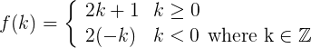
For the non-negative integers (0,1,2,3,…) the function maps to (1, 3, 5, 7,…) and for negative integers (-1, -2, -3,…), the corresponding piece-wise function maps to (2, 4, 6, 8,…). Thus all the integers are mapped to some natural number and there is no natural number that can’t be linked to an integral pre-image. The set of Integers (Z) , is therefore, CI.
A more intellectual challenge is to prove the set of Rational numbers (Q) to be CI. For doing so, several proofs exist. For the simplest method, we make use of an enumeration technique first showcased by Cantor. It provides a mechanism to generate or list all rational numbers one by one. Subsequently, we need to map them to the set of natural numbers.
In Figure 3, we observe the top row specifies all the integral values with alternating positive and negative numbers placed in the sequence. Below, we have the matrix-style listing of all possible rational values that can be generated by taking ‘a’ as the column header value and having different values of ‘b’ in a/b. Starting from 0, we can enumerate all rational numbers by traversing diagonally as depicted. Then, we can map this sample traversal sequence to the set of natural numbers with 0 mapped to 1, 1 mapped to 2, ½ mapped to 3, -1 mapped to 4 and so on.
Do note however, we still require a bijective function to establish sound mathematical basis of mapping each rational number to a unique natural number. To take a look at the proof and at the derivation of such a formula (interspersed with great humour!), please refer to this website [3].
 Fig. 3: Enumeration procedure for Rational numbers.
Uncountably Infinite Sets
Now, let’s bring our attention towards understanding the next logical question that arises in mind: We understand what Countable and Countably Infinite sets are. But what does Uncountability of sets mean? And the sequential question – what are uncountably infinite sets?
Following from the definition of Countability, an Uncountable Set is one for which no set T ⊂ N can be found to which it can be bijectively mapped to. It seems counter-intuitive when we think that if an infinite set such as that of integers can be mapped to N bijectively, what kind of trouble can we possibly encounter with any other set? Yet here’s where the ingenuity of George Cantor becomes evident. He showed how the elements of certain sets can’t be enumerated by using any Listing procedure. The most prominent example is the set of real numbers (ℝ).
The real number set can be thought of as the union of the set of all rational numbers and the set of all irrational numbers. For proving uncountability of real number sets in the most simple manner, a technique called Cantor’s diagonalization argument is used.
It’s a proof by contradiction. We first assume that a listing procedure exists for mapping all real numbers to natural numbers. By fleshing out the arguments based on this assumption, we arrive at a contradiction that proves the assumption as false thereby establishing the validity of the opposite claim that no listing procedure exists that can bijectively map the two sets.
To demonstrate the usage, let us consider the set of all real numbers between 1 and 2 as set ‘A’. We begin our analysis by assuming the existence of a listing procedure that maps all the members of ‘A’ to the set of ‘N’ which implies its Countability. The listing can be as shown in Figure 4.
 Fig. 4: The Listing of all the members of set ‘A’.
In Figure 4’s representation style, we specify each real number as ‘1.(decimal place) followed_by_the_fractional_part’. It’s advantageous to write in the above form as it properly represents the real numbers and helps demonstrate the technique. Note here that the fractional part is too large to be expressed, hence we add the three dots at the end. To understand the Listing procedure more clearly, we’ll consider a toy example after the explanation is complete.
To make the representation more generic, let’s write the fractional digits as follows:

Fig. 5: Real numbers written generically.
Diagonalization Procedure
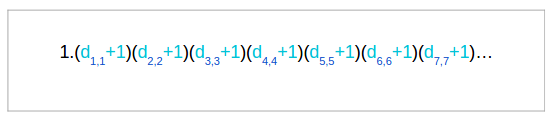
The technique aims to generate a real number that is not part of the listing. In order to find such a number, we begin by adding one to the first fractional digit of the first number (d1,1+1) in the listing. The sum obtained becomes the first fractional digit of the desired number. We then consider the second digit of the second number and add 1 to it (d2,2+1). We continue repeating the above addition by taking the nth fractional digit of the nth real number.

Fig. 6: Choosing the Diagonal elements from the listing.
The addition here is cyclic however. If the digit is 9, adding 1 should imply the output digit to be considered is 0. For rest of the digits (0 to 8), adding one produces the next sequential integral digit.
If we choose to represent the real numbers in equivalent binary, then instead of adding 1 as applied above, we compliment the nth bit of the nth number. Thus if d3,3 is 1, we make it 0 and use ahead.
Now, we compose the desired real number as follows:
In case we use the binary representation, the target number is composed of all the complemented bits.
To demonstrate diagonalization procedure, let’s consider the set B = {1.1, 1.2, 1.314, 1.4788, 1.5, 1.631192, 1.7, 1.8}. We note here at the onset that it’s a finite set and the number so obtained from the diagonalization is not going to be a member of this set. For the fractional part, we consider as many digits as there are members of the set. For B, every member’s fractional portion will be represented using 8 digits.

Fig. 7: The output real number from the Diagonalization procedure.
Coming back to the primary analysis, the obtained real number is distinct from all the numbers present in the listing as it differs from each number by at least one digit in its fractional portion. Yet, it is very much a part of set A (it is a real number between 1 and 2) but not part of the listing. It thus contradicts our initial assumption that the set is Countable as every member of the set is part of the listing. If the set is not Countable, it qualifies as an Uncountable set. Since infinitely many real number are possible between 1 and 2, we conclude that it is an Uncountably Infinite (UCI) set.
The conclusion that we can infer from the above result is that for the real number set ℝ, its cardinality is greater than that of Countably Infinite sets such as N. Despite both being infinite, the UCI set’s cardinality (called ‘Aleph-one’) is greater than that of a CI set. So an ordering between the cardinalities of the two sets can be established.
Aleph-one > Aleph-zero
The above result can be refined by considering the Cantor’s theorem.
Cantor’s theorem
Cantor’s theorem states that the power set of a set has a strictly greater cardinality than the concerned set which can be mathematically expressed as:

Power set of a set is the set of all its subsets which also includes the empty set {}. For a set A={1,2,4}, the power set of A will be: P(A) = { {}, {1}, {2},{4}, {1,2}, {1,4}, {2,4}, {1,2,4} }.
Surprisingly, the theorem is also applicable to the infinite sets. It relates the cardinalities of UCI and CI sets as follows:

or

The above result is indicative of UCI sets being infinitely larger than CI sets, thus establishing two orders of infinity.
Note: The above conclusions were originally arrived at by deploying more rigorous and formal mathematical analysis that forms the core content of Cantor’s and other mathematicians’ immense contribution to the field of mathematics. Yet much of it goes beyond the scope of this blogpost.
Examples of CI and UCI set
We arrived at the CI nature of the ensuing sets: Natural numbers (N), Integers (Z) and Rational numbers (Q). Yet which sets are UCI? We proved the real number set to be UCI. The sets of Irrational numbers and Complex numbers are also UCI. Figure 8 depicts an overview of CI and UCI classification of number sets.

Fig. 8: Hierarchical arrangement of number sets along with the CI/UCI notation.
In the figure, the shaded portion represents the Irrational numbers. The set of Real numbers can be thought of as the union of rational and irrational number sets. In fact, the Uncountable nature of real number set arises because of the presence of Irrational numbers within the set.
Application of CI/UCI concept to the field of Computer Science
Now that we’re well-versed with the crucial tenets of Modern set theory and the Countability concepts, an important question with reference to the domain of computer science must arise in our minds – Can this knowledge find application and utility? The answer, is ‘Yes!’.
In theoretical computer science, often the questions of finiteness of language sets and Turing Machine operation are answered using the CI/UCI concept. Also, the concept can be put to use to show that not all problems can be solved using computers [4] thus defining the limit of computational capabilities.
Conclusion
From our experiences with the principles of set theory, we have come to gain some understanding of what infinity means in a mathematical sense. The idea is fundamentally abstract, for the question of existence of infinite quantities in the physical universe has witnessed much debate and deliberation yet there are no clear answers. Scientists aren’t keen on seeking answers as well, for the concept finds more theoretical relevance than applicability to problems of contemporary times. Nonetheless, it constitutes an interesting field of study that has fascinated, and continues to fascinate, the curiosity of mankind.
For those interested in learning about Cantor’s set theory in a greater depth, you can make way to the highly detail intensive website at [5] that takes up the titular concern of this blog-post in a more detailed evaluation.
For a historical account of George Cantor’s mathematical legacy, refer to the link at [6].
References:
[1] Rich Schwartz, Countable and Uncountable Sets
[https://www.math.brown.edu/~res/MFS/handout8.pdf]
[2] Aleph-Null symbol extracted from Wikipedia
[https://en.wikipedia.org/wiki/Aleph_number#/media/File:Aleph0.svg]
[3] Coopertoons – Countability of Rational Numbers
[http://www.coopertoons.com/education/countingrationals/cantorsrationalnumbers.html]
[4] Dr. Abhijit Das, Chapter 4: Sizes of Sets
[http://cse.iitkgp.ac.in/~abhij/course/theory/DS/Autumn07/setsize.pdf]
[5] Alexander Bogomolny, Cut the Knot
[http://www.cut-the-knot.org/WhatIs/WhatIsInfinity.shtml]
[6] 19th Century Mathematics – Cantor
[http://www.storyofmathematics.com/19th_cantor.html]